Overview
csemGT estimates conditional standard errors of
measurement (CSEMs) under Generalizability Theory for the univariate
single-facet design in which persons are crossed with items (a
p $\times$ i design). Whereas a single overall SEM
summarises measurement precision for a whole test, a conditional SEM
describes how precision varies along the score scale, so that
examinees at different observed-score levels can be assigned different
error bands.
The package implements the absolute-error estimator and the three
relative-error estimators (full, large_a,
uncorrelated) developed by Brennan (1998), together with
optional polynomial smoothing of the conditional error variances across
the score scale and analytical or bootstrap standard errors for the
per-person estimates. csemGT is the R companion to the
Stata gtcsem command and reproduces its numerical
results.
This vignette walks through a minimal analysis. For the full argument
list see ?csem_gt; for replications of published examples
see the Examples vignette.
Installation
# install.packages("remotes")
remotes::install_github("rgempp/csemGT")
The mirt package is an optional dependency used only by
some of the worked examples in the Examples vignette; it is not
required for the core functionality shown here.
A minimal example
The package ships with iowa_like, a simulated
3000 $\times$ 40 matrix of dichotomously scored item
responses. It is not real test data: it was generated
from a Rasch model whose parameters were calibrated so that its
ANOVA-based mean error variances match the values Brennan (1998, p. 314)
reports for the ITED Vocabulary Test example. See
?iowa_like for the full provenance.
To keep the vignette fast we draw a reproducible subsample of 600 persons; the analysis is otherwise identical on the full matrix.
library(csemGT)
data(iowa_like)

set.seed(1998)
iowa_sub <- iowa_like[sample(nrow(iowa_like), 600), ]

fit <- csem_gt(iowa_sub, error_type = "relative", method = "full")
error_type = "relative" requests the relative
(-type)
conditional error variance, and method = "full" selects
Brennan’s finite-sample estimator (Equations 35–36), which is the
default. No bootstrap is requested, so standard errors are the
closed-form analytical approximation.
Inspecting the fit: print()
fit
#> ----------------------------------------------------------------
#> Conditional SEMs in Generalizability Theory
#> ----------------------------------------------------------------
#> Design          :  univariate single-facet (p x i, crossed)
#> Persons (n_p)   :  600
#> G-study items   :  40
#> D-study items   :  40
#> Method          :  full
#> SE method       :  analytical
#> Smoothing       :  quadratic on observed score
#> ANOVA table
#> ----------------------------------------------------------------
#>   Effect    df              SS              MS         sigma^2
#> ----------------------------------------------------------------
#>   p          599      958.459833        1.600100      0.035236
#>   i           39      359.446500        9.216577      0.015043
#>   pi       23361     4453.553500        0.190641      0.190641
#> D-study error variances and SEMs (n_i' = 40)
#> ----------------------------------------------------------------
#>   sigma^2(Delta) =   0.005142      sigma(Delta) = 0.071708  (absolute)
#>   sigma^2(delta) =   0.004766      sigma(delta) = 0.069036  (relative)
#> Reliability-like coefficients
#> ----------------------------------------------------------------
#>   Generalizability coef.    E rho^2     =   0.8809
#>   Dependability coef.       Phi         =   0.8727
#> Quadratic smoothing fits  (y = b0 + b1*score + b2*score^2)
#> --------------------------------------------------------------------------
#>   Quantity              b0         b1         b2        R^2       RMSE
#> --------------------------------------------------------------------------
#>   rel_ev_full           0.00036    0.02189   -0.02185     0.8843    0.00041
#> Mean variance of estimator across persons
#> ----------------------------------------------------------------
#>   Quantity              Analytical
#> ----------------------------------
#>   rel_ev_full         6.927086e-05
The printed report is organised in blocks. The header records the design and the estimation choices. The ANOVA table gives the person, item, and residual mean squares and the corresponding variance components. The D-study block reports the overall absolute and relative error variances and SEMs: here and , closely reproducing the values Brennan (1998) reports for the ITED Vocabulary Test and confirming that the 600-person subsample preserves the calibrated properties of the full dataset. The reliability-like coefficients (generalizability coefficient and dependability coefficient ) and the quadratic smoothing fit close the report.
Per-score view: summary()
summary(fit)
#> ----------------------------------------------------------------
#> Summary of Conditional SEMs in Generalizability Theory
#> ----------------------------------------------------------------
#> Paradigm     :  gt
#> Methods      :  full
#> Error types  :  relative
#> Persons      :  600
#> Items        :  40
#> Global statistics
#> ----------------------------------------------------------------
#>   Relative SEM   sigma(delta) = 0.069036     E rho^2 =   0.8809
#>   Absolute SEM   sigma(Delta) = 0.071708     Phi     =   0.8727
#> CSEM by observed score
#> ----------------------------------------------------------------
#>  observed_score group_size cum_freq percentile rel_full
#>           0.025          1   0.0017        0.2  0.03149
#>           0.050          1   0.0033        0.3  0.03583
#>           0.075          3   0.0083        0.8  0.04154
#>           0.100          1   0.0100        1.0  0.05019
#>           0.125          3   0.0150        1.5  0.05413
#>           0.150          5   0.0233        2.3  0.05393
#>           0.175          6   0.0333        3.3  0.06083
#>           0.200          7   0.0450        4.5  0.06183
#>           0.250          9   0.0600        6.0  0.06624
#>           0.275         11   0.0783        7.8  0.06930
#>           0.300         10   0.0950        9.5  0.06864
#>           0.325         14   0.1183       11.8  0.07128
#>           0.350         12   0.1383       13.8  0.07367
#>           0.375         17   0.1667       16.7  0.07514
#>           0.400         19   0.1983       19.8  0.07507
#>           0.425         18   0.2283       22.8  0.07627
#>           0.450         14   0.2517       25.2  0.07443
#>           0.475         19   0.2833       28.3  0.07709
#>           0.500         21   0.3183       31.8  0.07655
#>           0.525         25   0.3600       36.0  0.07675
#>           0.550         30   0.4100       41.0  0.07612
#>           0.575         27   0.4550       45.5  0.07559
#>           0.600         21   0.4900       49.0  0.07443
#>           0.625         20   0.5233       52.3  0.07267
#>           0.650         24   0.5633       56.3  0.07383
#>           0.675         32   0.6167       61.7  0.07136
#>           0.700         37   0.6783       67.8  0.07019
#>           0.725         31   0.7300       73.0  0.06916
#>           0.750         27   0.7750       77.5  0.06728
#>           0.775         21   0.8100       81.0  0.06498
#>           0.800         21   0.8450       84.5  0.06222
#>           0.825         24   0.8850       88.5  0.05991
#>           0.850         25   0.9267       92.7  0.05581
#>           0.875         15   0.9517       95.2  0.05198
#>           0.900         14   0.9750       97.5  0.04919
#>           0.925          7   0.9867       98.7  0.04368
#>           0.950          5   0.9950       99.5  0.03813
#>           0.975          2   0.9983       99.8  0.03257
#>           1.000          1   1.0000      100.0  0.01939
summary() adds the conditional SEM tabulated by observed
score, together with each score group’s size, cumulative frequency, and
percentile. Reading down the rel_full column shows the
characteristic concave pattern: the relative CSEM is small at the
extremes of the score scale, rises to a maximum near the middle, and
declines again — the same shape Brennan (1998, Figure 1d) obtained for
the fitted relative SEM of a dichotomously scored test.
Visualising: plot()
plot(fit)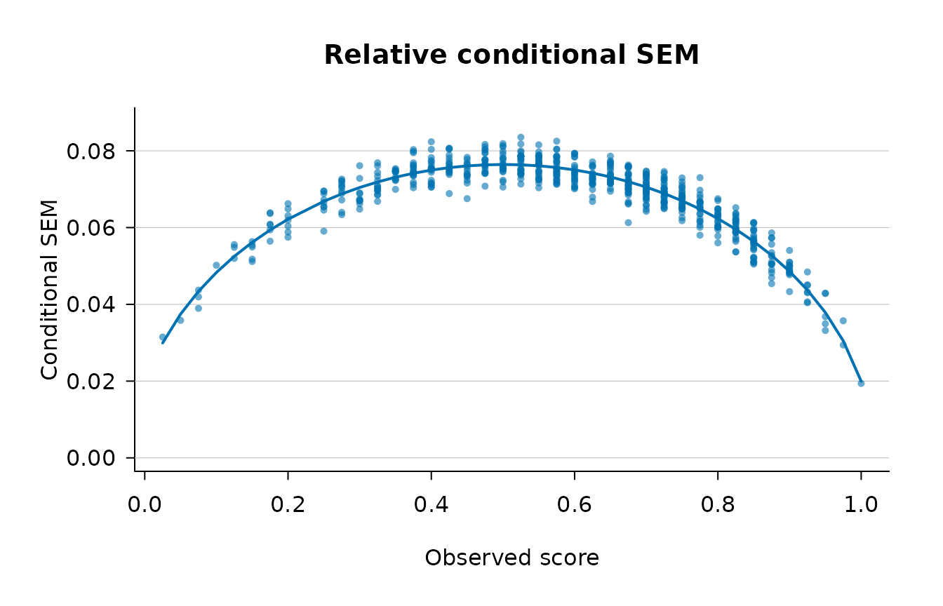
The default plot shows the per-person relative conditional SEM
against observed score, overlaid with the fitted quadratic smooth.
Additional layouts — comparing estimators in a single panel,
side-by-side panels, and analytical or bootstrap confidence bands — are
documented in ?plot.csem and demonstrated in the
Examples vignette.
The fitted object
csem_gt() returns an object of class
"csem". Its main components are the per-person estimates
($estimates), the by-score table ($by_score),
the G-study variance components ($variance_components), the
smoothing fits ($smooth_fits), and the smoother sample
diagnostics ($diagnostics). Convenience accessors are
provided:
str(fit, max.level = 1)
#> List of 15
#>  $ estimates          :'data.frame': 600 obs. of  13 variables:
#>  $ by_score           :'data.frame': 39 obs. of  10 variables:
#>  $ call               : language csem_gt(data = iowa_sub, method = "full", error_type = "relative")
#>  $ paradigm           : chr "gt"
#>  $ methods            : chr "full"
#>  $ error_types        : chr "relative"
#>  $ arguments          :List of 17
#>  $ variance_components:List of 6
#>  $ smooth_fits        :List of 1
#>  $ diagnostics        :List of 3
#>  $ bootstrap          : NULL
#>  $ scale_transform    : NULL
#>  $ n_persons          : int 600
#>  $ n_items            : int 40
#>  $ version            :Classes 'package_version', 'numeric_version'  hidden list of 1
#>  - attr(*, "class")= chr [1:2] "csem" "list"

# variance components
coef(fit)
#> $anova_table
#>        source    df        SS        MS
#> 1      person   599  958.4598 1.6000999
#> 2        item    39  359.4465 9.2165769
#> 3 person:item 23361 4453.5535 0.1906405
#>
#> $person
#> [1] 0.03523648
#>
#> $item
#> [1] 0.01504323
#>
#> $residual
#> [1] 0.1906405
#>
#> $population_quantities
#> $population_quantities$absolute_error_var
#> [1] 0.005142094
#>
#> $population_quantities$absolute_sem
#> [1] 0.0717084
#>
#> $population_quantities$relative_error_var
#> [1] 0.004766013
#>
#> $population_quantities$relative_sem
#> [1] 0.06903632
#>
#>
#> $reliability_coefficients
#> $reliability_coefficients$erho2
#> [1] 0.8808571
#>
#> $reliability_coefficients$phi
#> [1] 0.8726529
#>
#> $reliability_coefficients$phi_lambda
#> [1] NA

# by-score table as a data frame
head(by_score(fit))
#>   observed_score group_size     cov_xim csem_var.relative_full
#> 1          0.025          1 0.000232906           0.0009915028
#> 2          0.050          1 0.006277778           0.0012836831
#> 3          0.075          3 0.008618946           0.0017291995
#> 4          0.100          1 0.003452991           0.0025185403
#> 5          0.125          3 0.005138889           0.0029325584
#> 6          0.150          5 0.014850427           0.0029124661
#>   csem.relative_full csem_var.analytic.relative_full se.analytic.relative_full
#> 1         0.03148814                    0.0002956770                0.01719526
#> 2         0.03582852                    0.0002283776                0.01511217
#> 3         0.04153760                    0.0001710728                0.01306453
#> 4         0.05018506                    0.0001164025                0.01078900
#> 5         0.05413089                    0.0001003035                0.01001091
#> 6         0.05392755                    0.0001012605                0.01005525
#>   ci_low.analytic.relative_full ci_up.analytic.relative_full
#> 1                   0.000000000                   0.06519023
#> 2                   0.006209218                   0.06544783
#> 3                   0.015931588                   0.06714361
#> 4                   0.029039007                   0.07133111
#> 5                   0.034509874                   0.07375191
#> 6                   0.034219631                   0.07363548
#>   smoothed_csem.relative_full
#> 1                  0.02994060
#> 2                  0.03745157
#> 3                  0.04337611
#> 4                  0.04830156
#> 5                  0.05250982
#> 6                  0.05616233
Next steps
-
?csem_gtdocuments every argument, including bootstrap options, polynomial smoothing, extreme-score handling, and then_items_DD-study generalisation. - The Examples vignette replicates published analyses, including a multi-panel comparison of the relative-error estimators.
- The Stata
gtcsemcommand produces the same estimates for users working in that environment.